Quickstart Tutorial
This is a “quickstart” tutorial for NMRPy in which an Agilent (Varian) NMR dataset will be processed. The following topics are explored:
This tutorial will use the test data in the nmrpy install directory:
site-packages/nmrpy/tests/test_data/test1.fid
The dataset consists of a time array of spectra of the phosphoglucose isomerase reaction:
fructose-6-phosphate -> glucose-6-phosphate
An example Jupyter notebook is provided in the docs subdirectory of
the nmrpy install directory, which mirrors this Quickstart Tutorial.
site-packages/nmrpy/docs/quickstart_tutorial.ipynb
Importing
The basic NMR project object used in NMRPy is the
FidArray, which consists of a set of
Fid objects, each representing a single spectrum in
an array of spectra.
The simplest way to instantiate an FidArray is by
using the from_path() method, and specifying
the path of the .fid directory:
>>> import nmrpy
>>> import os
>>> fname = os.path.join(os.path.dirname(nmrpy.__file__),
                         'tests', 'test_data', 'test1.fid')
>>> fid_array = nmrpy.from_path(fname)
You will notice that the fid_array object is instantiated and now owns
several attributes, most of which are of the form fidXX where XX is
a number starting at 00. These are the individual arrayed
Fid objects.
Apodisation and Fourier-transformation
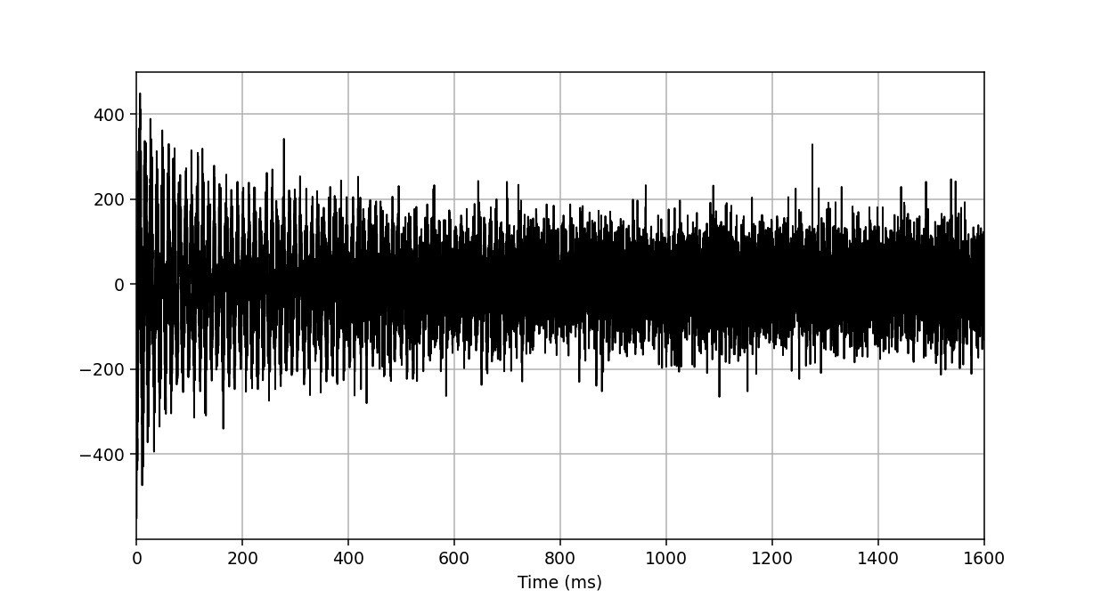
To quickly visualise the imported data, we can use the plotting functions owned
by each Fid instance. This will not display the
imaginary portion of the data:
>>> fid_array.fid00.plot_ppm()
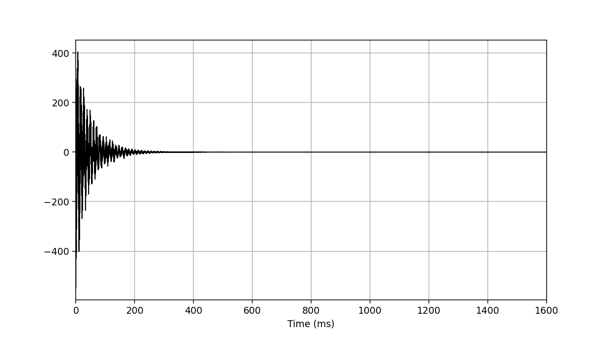
We now perform apodisation of the FIDs using the default value of 5 Hz, and visualise the result:
>>> fid_array.emhz_fids()
>>> fid_array.fid00.plot_ppm()
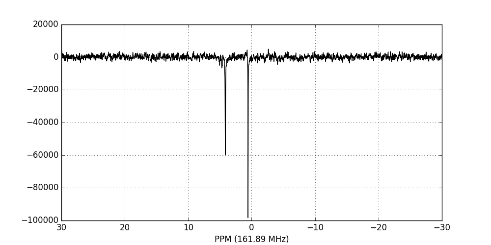
Finally, we zero-fill and Fourier-transform the data into the frequency domain:
>>> fid_array.zf_fids()
>>> fid_array.ft_fids()
>>> fid_array.fid00.plot_ppm()
Phase-correction
It is clear from the data visualisation that at this stage the spectra require
phase-correction. NMRPy provides a number of GUI widgets for manual processing
of data. In this case we will use the phaser()
method on fid00:
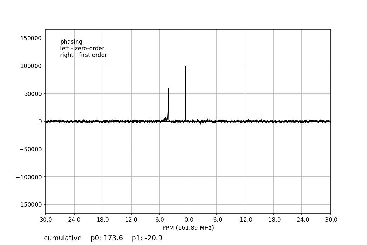
>>> fid_array.fid00.phaser()
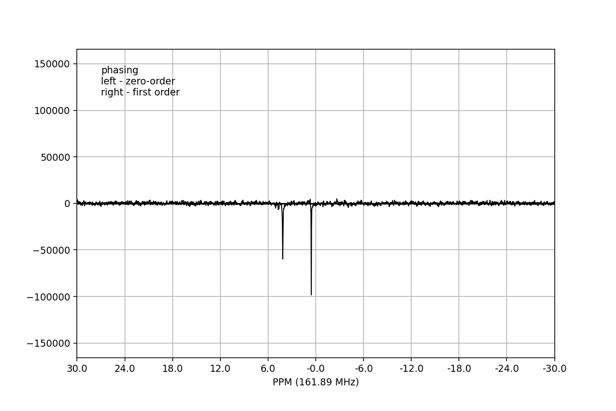
Dragging with the left mouse button and right mouse button will apply zero- and
first-order phase-correction, respectively. The cumulative phase correction for
the zero-order (p0) and first-order (p1) phase angles is displayed at
the bottom of the plot so that these can be applied programatically to all
Fid objects in the
FidArray using the
ps_fids() method.
Alternatively, automatic phase-correction can be applied at either the
FidArray or Fid
level. We will apply it to the whole array:
>>> fid_array.phase_correct_fids()
And plot an array of the phase-corrected data:
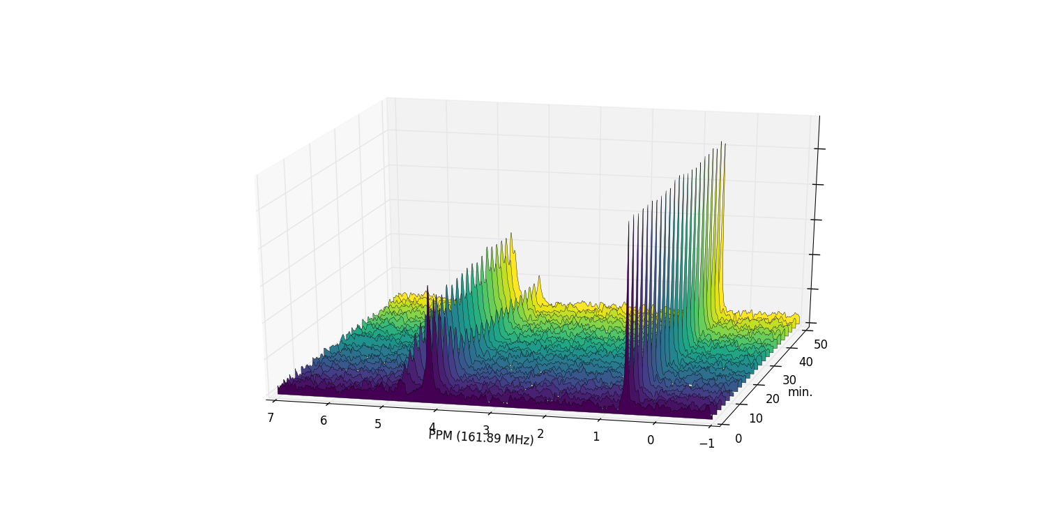
>>> fid_array.plot_array()
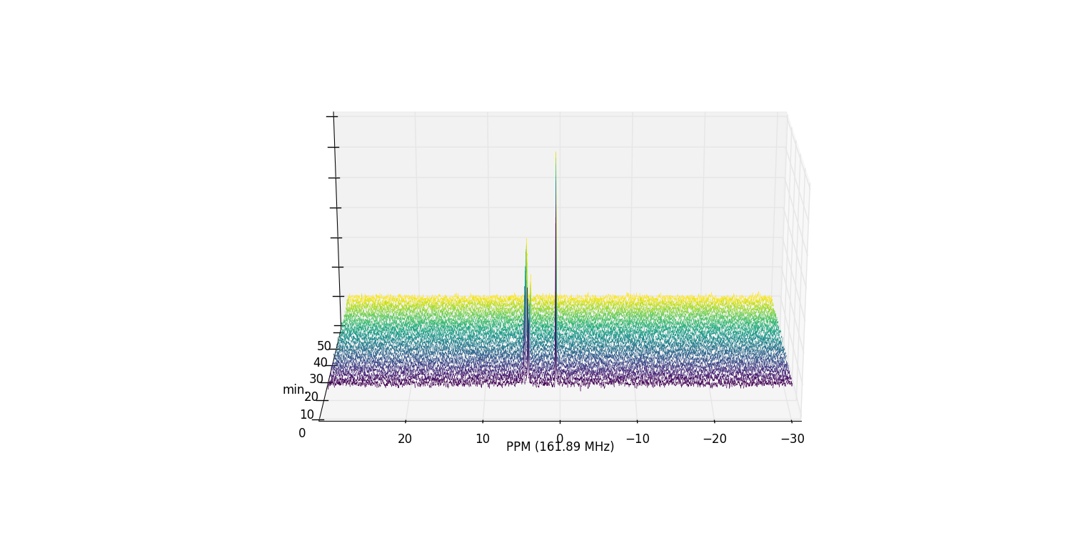
Zooming in on the relevant peaks, changing the view perspective, and filling the spectra produces a more interesting plot:
>>> fid_array.plot_array(upper_ppm=7, lower_ppm=-1, filled=True, azim=-76, elev=23)
At this stage it is useful to discard the imaginary component of our data, and
possibly normalise the data (by the maximum data value amongst the
Fid objects):
>>> fid_array.real_fids()
>>> fid_array.norm_fids()
Calibration
The spectra may need calibration by assigning a chemical shift to a
reference peak of a known standard and adjusting the spectral offset
accordingly. To this end, a
calibrate() convenience method exists that
allows the user to easily select a peak and specify the PPM. This method can be
applied at either the FidArray or
Fid level. We will apply it to the whole array:
>>> fid_array.calibrate()
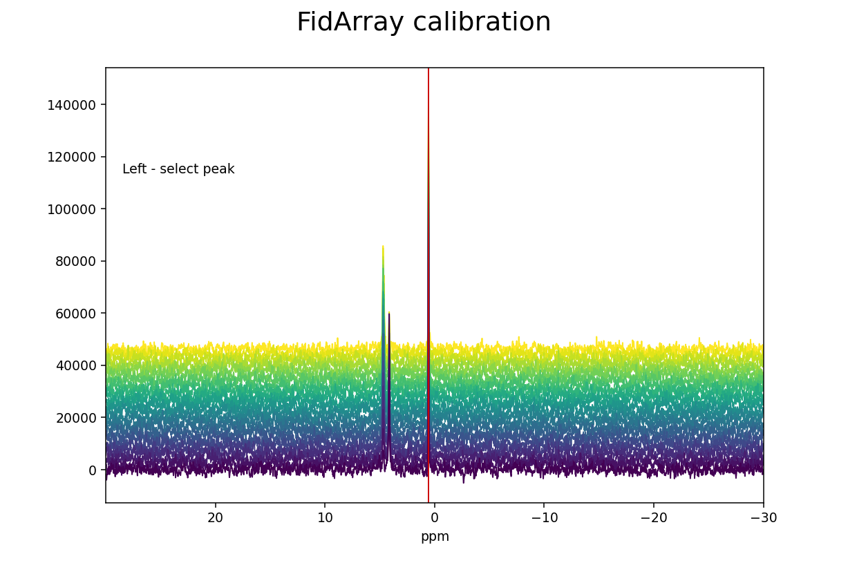
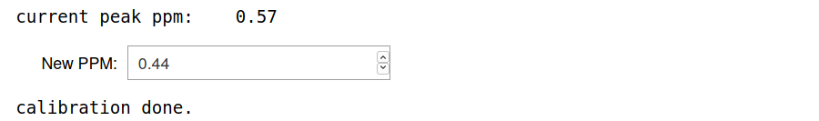
Left-clicking selects a peak and its current ppm value is displayed below
the spectrum. The new ppm value can be entered in a text box, and hitting
Enter completes the calibration process. Here we have chosen triethyl
phosphate (TEP) as reference peak and assigned its chemical shift value of 0.44
ppm (the original value was 0.57 ppm, and the offset of all the spectra in the
array has been adjusted by 0.13 ppm after the calibration).
Peak-picking
To begin the process of integrating peaks by deconvolution, we will need to
pick some peaks. The peaks attribute of a
Fid is an array
of peak positions, and ranges is an array of
range boundaries. These two objects are used in deconvolution to integrate the
data by fitting Lorentzian/Gaussian peak shapes to the spectra.
peaks and ranges
may be specified programatically, or picked using the interactive GUI widget:
>>> fid_array.peakpicker(fid_number=10)
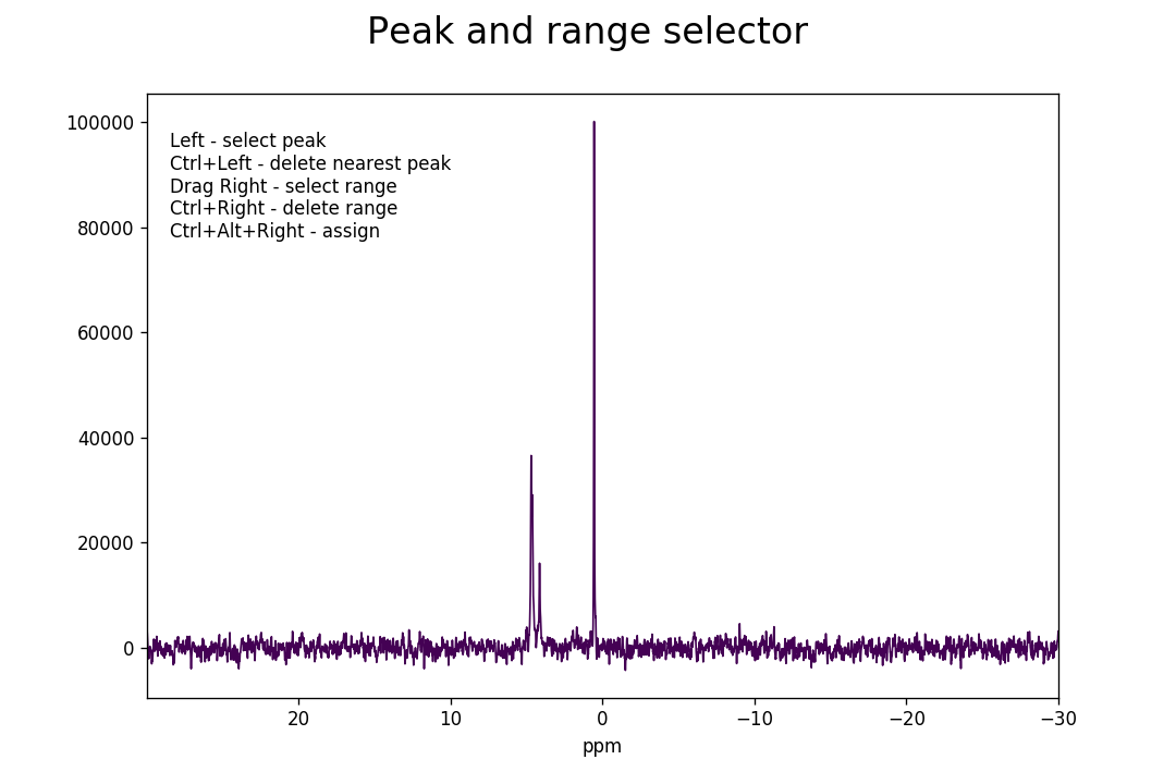
Left-clicking specifies a peak selection with a vertical red line. Dragging with a right-click specifies a range to fit independently with a grey rectangle:
Inadvertent wrongly selected peaks can be deleted with Ctrl+left-click; wrongly
selected ranges can be deleted with Ctrl+right-click. Once you are done
selecting peaks and ranges, these need to be assigned to the
FidArray; this is achieved with a
Ctrl+Alt+right-click.
Ranges divide the data into smaller portions, which significantly speeds up the process of fitting of peakshapes to the data. Range-specification also prevents incorrect peaks from being fitted by the fitting algorithm.
Having used the peakpicker()
FidArray method (as opposed to the
peakpicker() on each individual
Fid instance), the peak and range selections have
now been assigned to each Fid in the array:
>>> print(fid_array.fid00.peaks)
[ 4.73  4.63  4.15  0.55]
>>> print(fid_array.fid00.ranges)
[[ 5.92  3.24]
 [ 1.19 -0.01]]
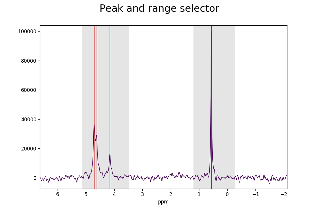
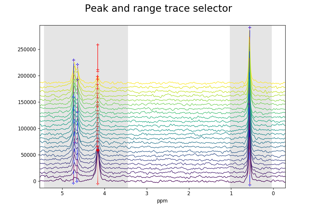
Peak-picking trace selector
Sometimes peaks are subject to drift so that the chemical shift changes over
time; this can happen, e.g., when the pH of the reaction mixture changes as the
reaction proceeds. NMRPy offers a convenient trace selector, with which the
drift of the peaks can be traced over time and the chemical shift selected
accordingly as appropriate for the particular Fid.
>>> fid_array.peakpicker_traces(voff=0.08)
As for the peakpicker(), ranges are selected
by dragging the right mouse button and can be deleted with Ctrl+right-click. A
peak trace is initiated by left-clicking below the peak underneath the first
Fid in the series. This selects a point and anchors the trace line, which is
displayed in red as the mouse is moved. The trace will attempt to follow
the highest peak. Further trace points can be added by repeated left-clicking,
thus tracing the peak through the individual Fids in the series. It is not
necessary to add an anchor point for every Fid, only when the trace needs to
change direction. Once the trace has traversed all the Fids, select a final
trace point (left-click) and then finalize the trace with a right-click. The trace will
change colour from red to blue to indicate that it has been finalized.
Additional peaks can then be selected by initiating a new trace. Wrongly selected traces can be deleted by Ctrl+left-click at the bottom of the trace that should be removed. Note that the interactive buttons on the matplotlib toolbar for the figure can be used to zoom and pan into a region of interest of the spectra.
As previously, peaks and ranges need to be assigned to the
FidArray with Ctrl+Alt+right-click. As can be seen
below, the individual peaks have different chemical shifts for the different
Fids, although the drift in these spectra is not significant so that
peakpicker_traces() need not have been used
and peakpicker() would have been sufficient.
This is merely for illustrative purposes.
>>> print(p.fid00.peaks)
[4.73311164 4.65010807 0.55783899 4.15787759]
>>> print(p.fid10.peaks)
[4.71187817 4.6404565  0.5713512  4.16366854]
>>> print(p.fid20.peaks)
[4.73311164 4.63466555 0.57907246 4.16366854]
Deconvolution
Individual Fid objects can be deconvoluted with
deconv(). FidArray
objects can be deconvoluted with
deconv_fids(). By default this is a
multiprocessed method (mp=True), which will fit pure Lorentzian lineshapes
(frac_gauss=0.0) to the peaks and
ranges specified in each
Fid.
We shall fit the whole array at once:
>>> fid_array.deconv_fids()
And visualise the deconvoluted spectra:
>>> fid_array.fid10.plot_deconv()
Zooming-in to a set of peaks makes clear the fitting result:
>>> fid_array.fid10.plot_deconv(upper_ppm=5.5, lower_ppm=3.5)
>>> fid_array.fid10.plot_deconv(upper_ppm=0.9, lower_ppm=0.2)
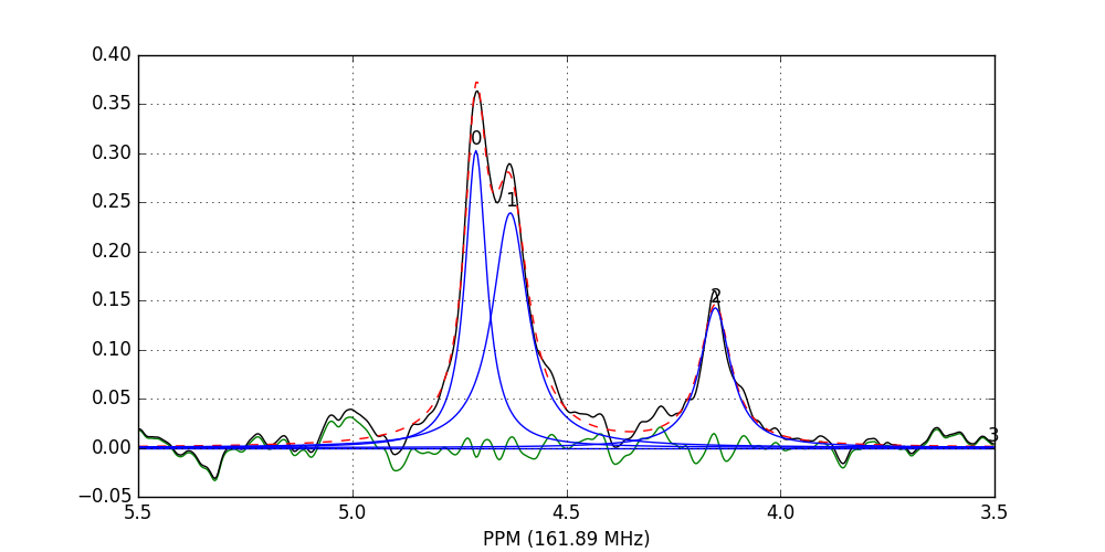
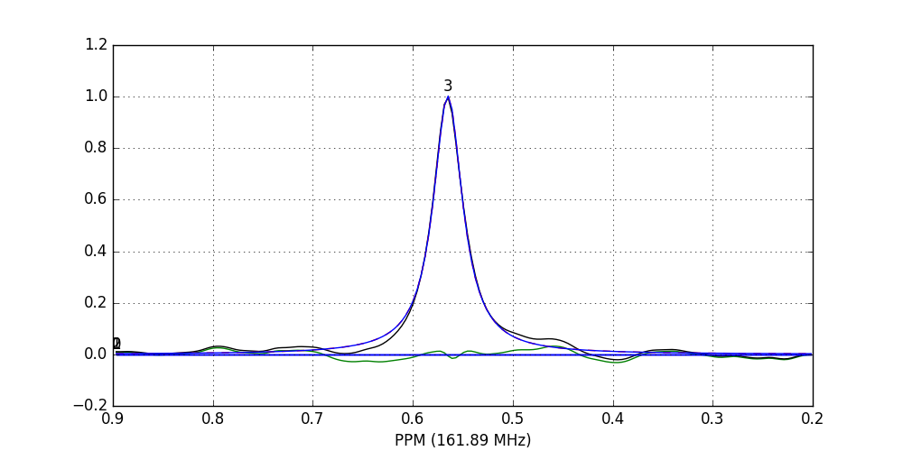
The lines are colour-coded according to:
- Blue: individual peak shapes (and peak numbers above);
- Black: original data;
- Red: summed peak shapes;
- Green: residual (original data - summed peakshapes).
In this case, peaks 0 and 1 belong to glucose-6-phosphate, peak 2 belongs to fructose-6-phosphate, and peak 3 belongs to triethyl-phosphate.
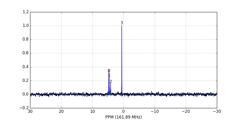
We can view the deconvolution result for the whole array using
plot_deconv_array(). Fitted peaks appear in
red:
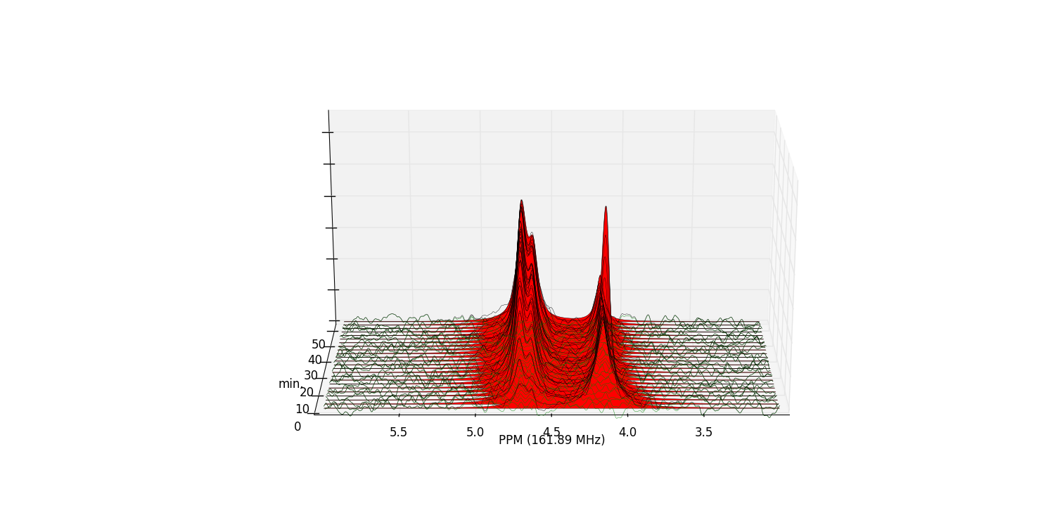
>>> fid_array.plot_deconv_array(upper_ppm=6, lower_ppm=3)
Peak integrals of the entire FidArray are stored in
deconvoluted_integrals, or in each
individual Fid as
deconvoluted_integrals.
Plotting the time-course
The acquisition times for the individual Fid
objects in the FidArray are stored in an array
t for easy access. Note that when each
Fid is collected with multiple transients/scans on
the spectrometer, the acquisition time is calculated as the middle of its
overall acquisition period.
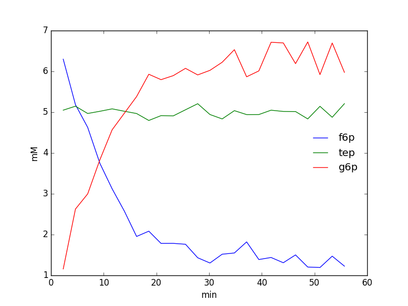
We could thus easily plot the time-course of the species integrals using the following code:
from matplotlib import pyplot as plt

integrals = fid_array.deconvoluted_integrals.transpose()

g6p = integrals[0] + integrals[1]
f6p = integrals[2]
tep = integrals[3]

#scale species by internal standard tep (5 mM)
g6p = 5.0*g6p/tep.mean()
f6p = 5.0*f6p/tep.mean()
tep = 5.0*tep/tep.mean()

species = {'g6p': g6p,
           'f6p': f6p,
           'tep': tep}

fig = plt.figure()
ax = fig.add_subplot(111)
for k, v in species.items():
    ax.plot(fid_array.t, v, label=k)

ax.set_xlabel('min')
ax.set_ylabel('mM')
ax.legend(loc=0, frameon=False)

plt.show()
Deleting individual Fid objects from a FidArray
Sometimes it may be desirable to remove one or more
Fid objects from a
FidArray, e.g. to remove outliers from the
time-course of concentrations. This can be conveniently achieved with the
del_fid() method, which takes as argument
the id of the Fid
to be removed. The acquisition time array
t is updated accordingly by removing the
corresponding time-point. After this,
deconv_fids() has to be run again to update
the array of peak integrals.
A list of all the Fid objects in a
FidArray is returned by the
get_fids() method.
>>> print([f.id for f in fid_array.get_fids()])
    ['fid00', 'fid01', 'fid02', 'fid03', 'fid04', 'fid05', 'fid06', 'fid07',
     'fid08', 'fid09', 'fid10', 'fid11', 'fid12', 'fid13', 'fid14', 'fid15',
     'fid16', 'fid17', 'fid18', 'fid19', 'fid20', 'fid21', 'fid22', 'fid23']

>>> for fid_id in [f.id for f in fid_array.get_fids()][::4]:
        fid_array.del_fid(fid_id)

>>> print([f.id for f in fid_array.get_fids()])
    ['fid01', 'fid02', 'fid03', 'fid05', 'fid06', 'fid07', 'fid09', 'fid10',
     'fid11', 'fid13', 'fid14', 'fid15', 'fid17', 'fid18', 'fid19', 'fid21',
     'fid22', 'fid23']

>>> print(['{:.2f}'.format(i) for i in fid_array.t])
    ['3.48', '5.80', '8.12', '12.76', '15.08', '17.40', '22.04', '24.36', '26.68',
     '31.32', '33.64', '35.96', '40.60', '42.92', '45.24', '49.88', '52.20', '54.52']
The gaps left by the deleted Fid objects are clearly visible in the plotted
FidArray:
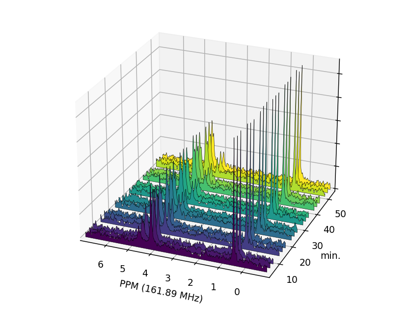
>>> fid_array.plot_array(upper_ppm=7, lower_ppm=-1, filled=True, azim=-68, elev=25)
Saving / Loading
The current state of any FidArray object can be
saved to file using the save_to_file() method:
>>> fid_array.save_to_file(filename='fidarray.nmrpy')
The filename need not be specified, if not given the name is taken from
fid_path and the .nmrpy extension is
appended. If the file exists, it is not overwritten; a forced overwrite can
be specified with:
>>> fid_array.save_to_file(filename='fidarray.nmrpy', overwrite=True)
The FidArray can be reloaded using
from_path():
>>> fid_array = nmrpy.from_path(fid_path='fidarray.nmrpy')
Full tutorial script
The full script for the quickstart tutorial:
import nmrpy
import os
from matplotlib import pyplot as plt

fname = os.path.join(os.path.dirname(nmrpy.__file__), 'tests',
                     'test_data', 'test1.fid')
fid_array = nmrpy.from_path(fid_path=fname)
fid_array.emhz_fids()
#fid_array.fid00.plot_ppm()
fid_array.ft_fids()
#fid_array.fid00.plot_ppm()
#fid_array.fid00.phaser()
fid_array.phase_correct_fids()
#fid_array.fid00.plot_ppm()
fid_array.real_fids()
fid_array.norm_fids()
#fid_array.plot_array()
#fid_array.plot_array(upper_ppm=7, lower_ppm=-1, filled=True, azim=-76, elev=23)
#fid_array.calibrate()

peaks = [ 4.73,  4.63,  4.15,  0.55]
ranges = [[ 5.92,  3.24], [ 1.19, -0.01]]
for fid in fid_array.get_fids():
    fid.peaks = peaks
    fid.ranges = ranges

fid_array.deconv_fids()

#fid_array.fid10.plot_deconv(upper_ppm=5.5, lower_ppm=3.5)
#fid_array.fid10.plot_deconv(upper_ppm=0.9, lower_ppm=0.2)
#fid_array.plot_deconv_array(upper_ppm=6, lower_ppm=3)

integrals = fid_array.deconvoluted_integrals.transpose()

g6p = integrals[0] + integrals[1]
f6p = integrals[2]
tep = integrals[3]

#scale species by internal standard tep at 5 mM
g6p = 5.0*g6p/tep.mean()
f6p = 5.0*f6p/tep.mean()
tep = 5.0*tep/tep.mean()

species = {'g6p': g6p,
           'f6p': f6p,
           'tep': tep}

fig = plt.figure()
ax = fig.add_subplot(111)
for k, v in species.items():
    ax.plot(fid_array.t, v, label=k)
ax.set_xlabel('min')
ax.set_ylabel('mM')
ax.legend(loc=0, frameon=False)
plt.show()

print([f.id for f in fid_array.get_fids()])

#delete selected Fids from array
for fid_id in [f.id for f in fid_array.get_fids()][::4]:
    fid_array.del_fid(fid_id)
print([f.id for f in fid_array.get_fids()])
print(['{:.2f}'.format(i) for i in fid_array.t])
#fid_array.plot_array(upper_ppm=7, lower_ppm=-1, filled=True, azim=-68, elev=25)

#fid_array.save_to_file(filename='fidarray.nmrpy')
#fid_array = nmrpy.from_path(fid_path='fidarray.nmrpy')