Quickstart Tutorial
This is a “quickstart” tutorial for NMRPy in which an Agilent (Varian) NMR dataset will be processed. The following topics are explored:
This tutorial will use the test data in the nmrpy install directory:
nmrpy/tests/test_data/test1.fid
The dataset consists of a time array of spectra of the phosphoglucose-isomerase reaction:
fructose-6-phosphate -> glucose-6-phosphate
Importing
The basic NMR project object used in NMRPy is the
FidArray, which consists of a set of
Fid objects, each representing a single spectrum in
an array of spectra.
The simplest way to instantiate an FidArray is by
using the from_path() method, and specifying
the path of the .fid directory:
import nmrpy
fid_array = nmrpy.data_objects.FidArray.from_path(fid_path='./tests/test_data/test1.fid')
You will notice that the fid_array object is instantiated and now owns
several attributes, amongst others, which are of the form fidXX where XX is
a number starting at 00. These are the individual arrayed
Fid objects.
Apodisation and Fourier-transformation
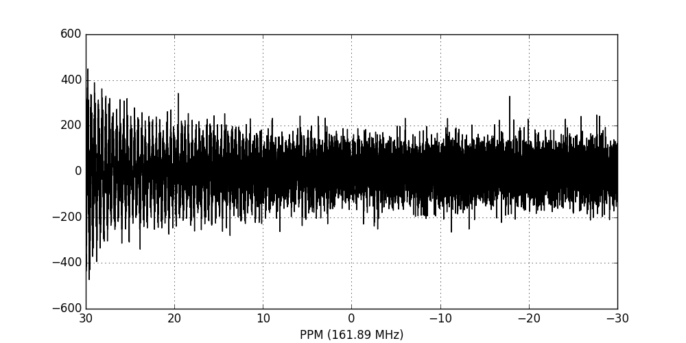
To quickly visualise the imported data, we can use the plotting functions owned
by each Fid instance. This will not display the
imaginary portion of the data:
fid_array.fid00.plot_ppm()
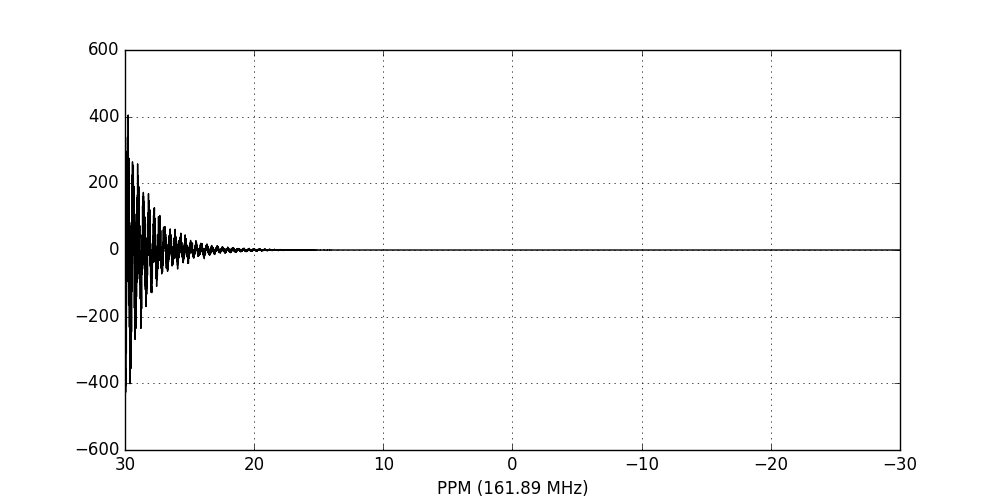
We now perform apodisation of the FIDs using the default value of 5 Hz, and visualise the result:
fid_array.emhz_fids()
fid_array.fid00.plot_ppm()
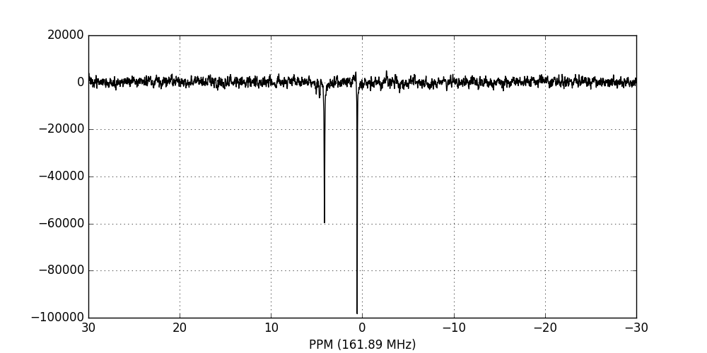
Finally, we Fourier-transform the data into the frequency domain:
fid_array.ft_fids()
fid_array.fid00.plot_ppm()
Phase-correction
It is clear from the data visualisation that at this stage the spectra require
phase-correction. NMRPy provides a number of GUI widgets for manual processing
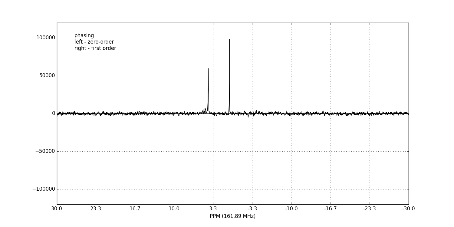
of data. In this case we will use the phaser()
method on fid00:
fid_array.fid00.phaser()
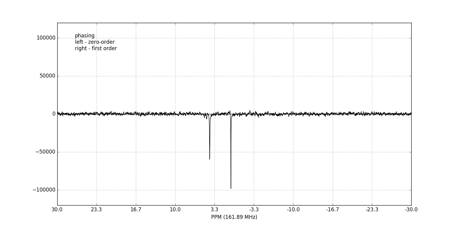
Dragging with the left mouse button and right mouse button will apply zero- and first-order phase-correction respectively.
Alternatively, automatic phase-correction can be applied at either the
FidArray or Fid
level. We will apply it to the whole array:
fid_array.phase_correct_fids()
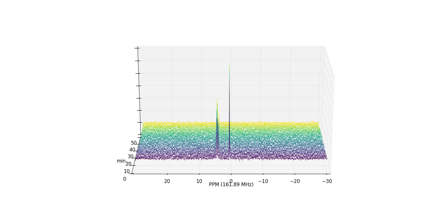
And plot an array of the phase-corrected data:
fid_array.plot_array()
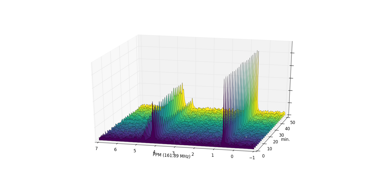
Zooming in on the relevant peaks, and filling the spectra produces a more interesting plot:
fid_array.plot_array(upper_ppm=7, lower_ppm=-1, filled=True, azim=-76, elev=23)
At this stage it is useful to discard the imaginary component of our data, and
possibly normalise the data (by the maximum data value amongst the
Fid objects):
fid_array.real_fids()
fid_array.norm_fids()
Peak-picking
To begin the process of integrating peaks by deconvolution, we will need to
pick some peaks. The peaks object is an array
of peak positions, and ranges is an array of
range boundaries. These two objects are used in deconvolution to integrate the
data by fitting Lorentzian/Gaussian peakshapes to the spectra.
peaks may be specified programatically, or
picked using the interactive GUI widget:
fid_array.peakpicker(fid_number=10)
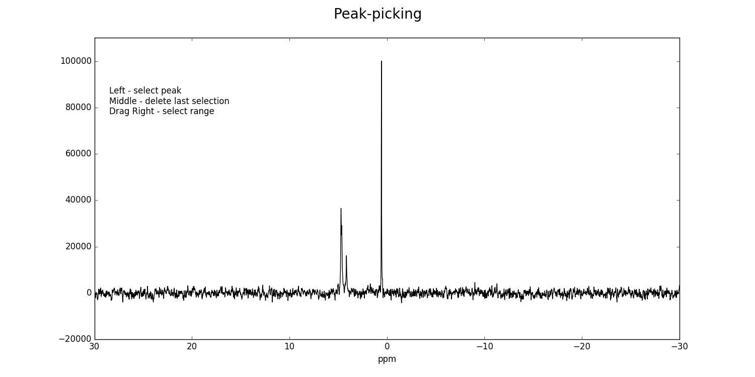
Left-clicking specifies a peak selection with a vertical red line. Dragging with a right-click specifies a range to fit independently with a grey rectangle:
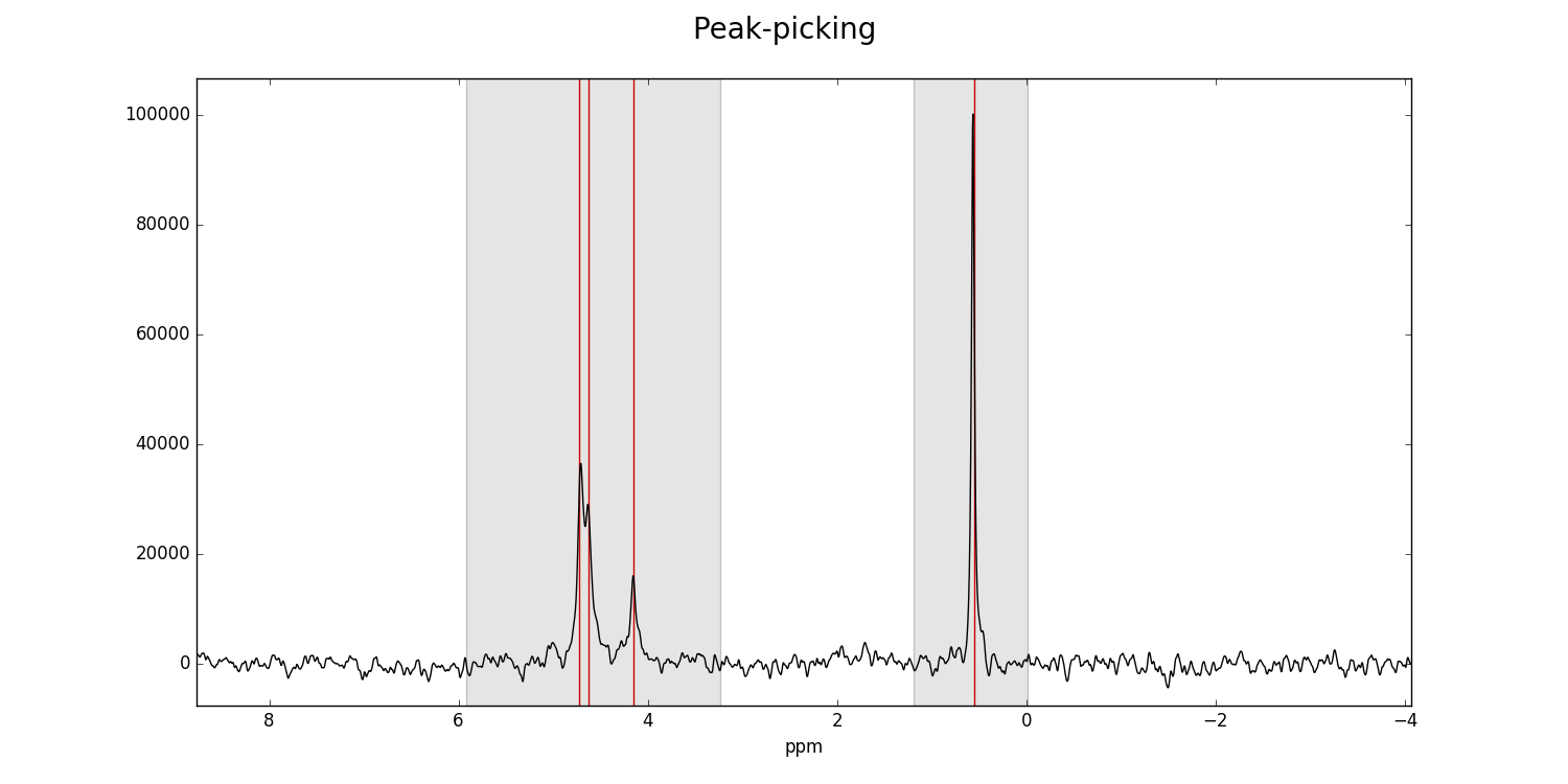
Ranges divide the data into smaller portions, which significantly speeds up the process of fitting of peakshapes to the data. Range-specification also prevents incorrect peaks from being fitted by the fitting algorithm.
Having used the peakpicker()
FidArray method (as opposed to the
peakpicker() on each individual
Fid instance), the peak and range selections have
now been assigned to each Fid in the array:
print(fid_array.fid00.peaks)
[ 4.73  4.63  4.15  0.55]
print(fid_array.fid00.ranges)
[[ 5.92  3.24]
 [ 1.19 -0.01]]
Deconvolution
Individual Fid objects can be deconvoluted with
deconv(). FidArray
objects can be deconvoluted with
deconv_fids(). By default this is a
multiprocessed method (mp=True), which will fit pure Lorentzian lineshapes
(frac_gauss=0.0) to the peaks and
ranges specified in each
Fid.
We shall fit the whole array at once:
fid_array.deconv_fids()
And visualise the deconvoluted spectra:
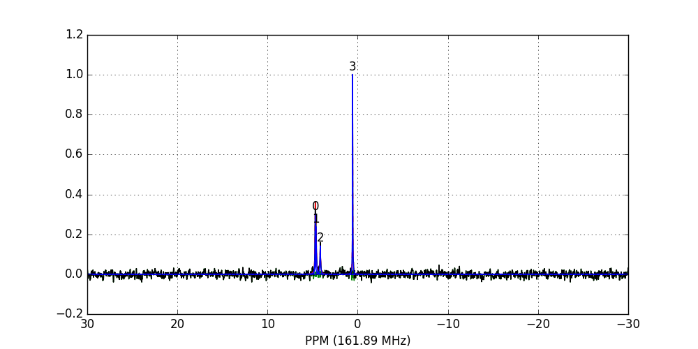
fid_array.fid10.plot_deconv()
Zooming-in to a set of peaks makes clear the fitting result:
fid_array.fid10.plot_deconv(upper_ppm=5.5, lower_ppm=3.5)
fid_array.fid10.plot_deconv(upper_ppm=0.9, lower_ppm=0.2)
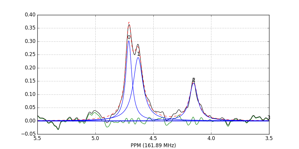
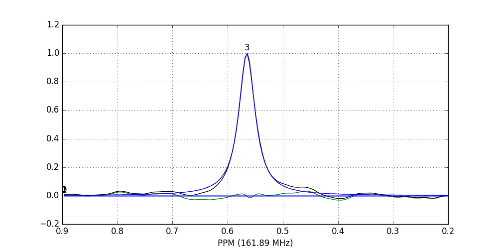
Black: original data; blue: individual peak shapes (and peak numbers above); red: summed peak shapes; green: residual (original data - summed peakshapes)
In this case, peaks 0 and 1 belong to glucose-6-phosphate, peak 2 belongs to fructose-6-phosphate, and peak 3 belongs to triethyl-phosphate.
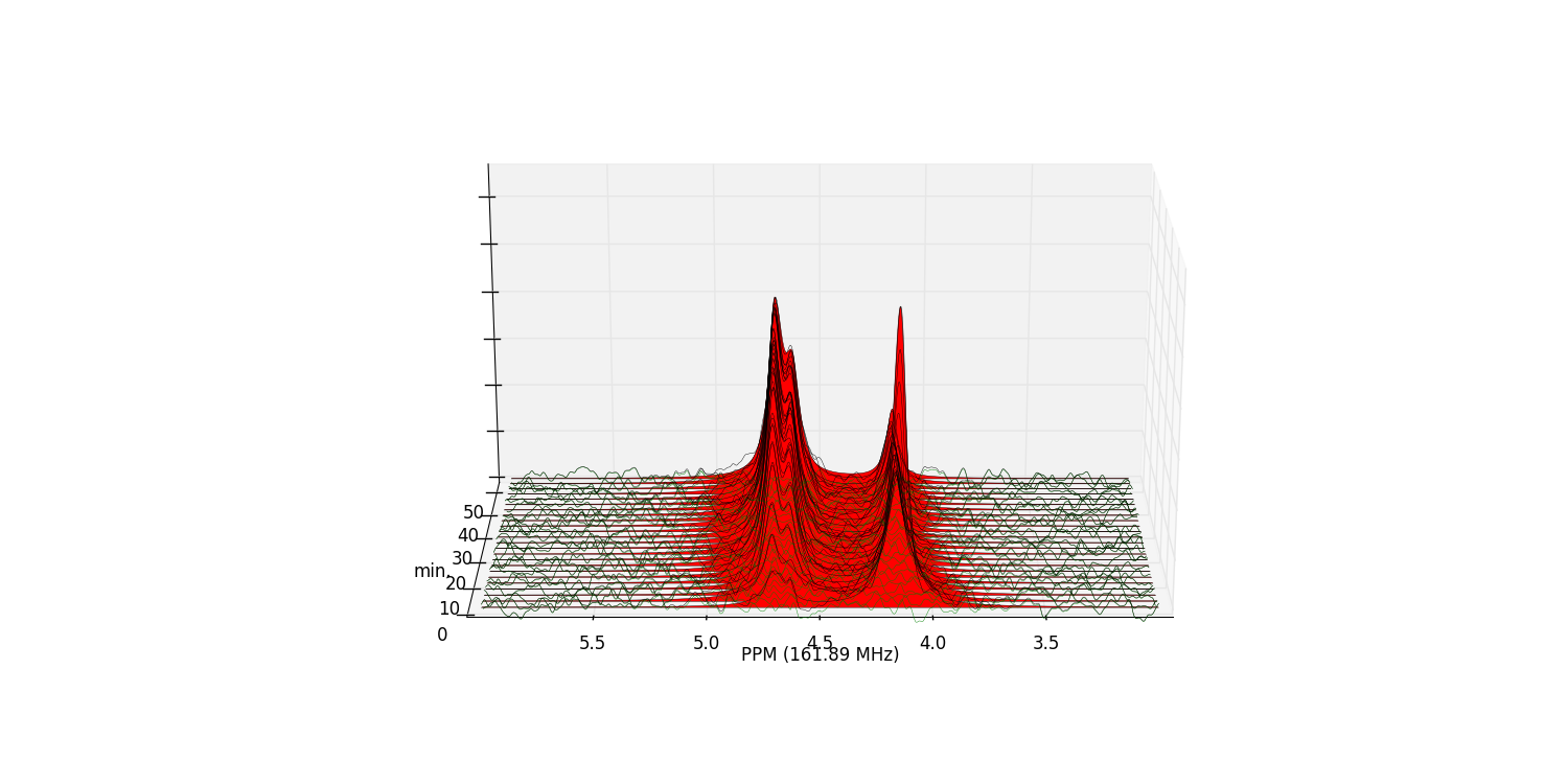
We can view the deconvolution result for the whole array using
plot_deconv_array(). Fitted peaks appear in
red:
fid_array.plot_deconv_array(upper_ppm=6, lower_ppm=3)
Peak integrals of the array are stored in
nmrpy.data_objects.FidArray.deconvoluted_integrals, or in each
individual Fid as
nmrpy.data_objects.Fid.deconvoluted_integrals.
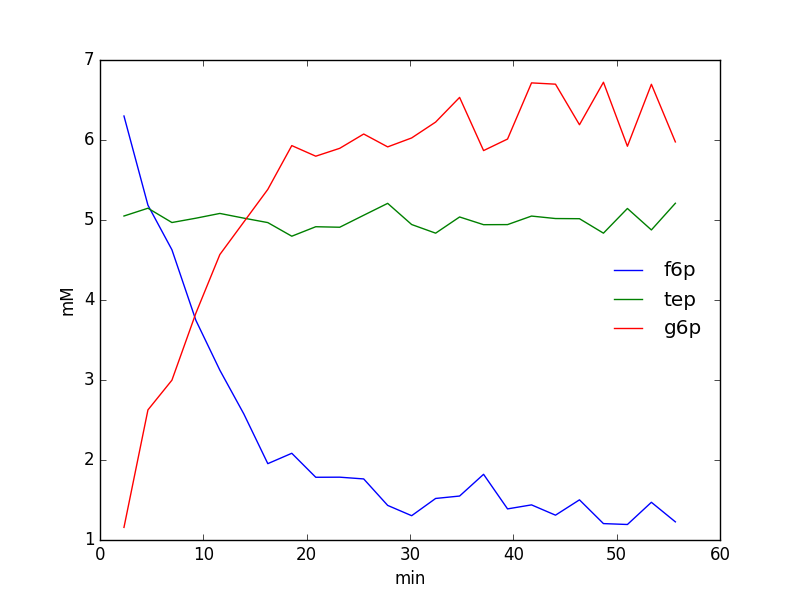
We could easily plot the species integrals using the following code:
import pylab

 integrals = fid_array.deconvoluted_integrals.transpose()

 g6p = integrals[0] + integrals[1]
 f6p = integrals[2]
 tep = integrals[3]

 #scale species by internal standard tep
 g6p = 5.0*g6p/tep.mean()
 f6p = 5.0*f6p/tep.mean()
 tep = 5.0*tep/tep.mean()

 species = {'g6p': g6p,
            'f6p': f6p,
            'tep': tep}

 fig = pylab.figure()
 ax = fig.add_subplot(111)
 for k, v in species.items():
     ax.plot(fid_array.t, v, label=k)

 ax.set_xlabel('min')
 ax.set_ylabel('mM')
 ax.legend(loc=0, frameon=False)

 pylab.show()
Exporting/Importing
The current state of any FidArray object can be
saved to file using the save_to_file() method:
fid_array.save_to_file(filename='fidarray.nmrpy')
And reloaded using from_path():
fid_array = nmrpy.data_objects.FidArray.from_path(fid_path='fidarray.nmrpy')
Full tutorial script
The full script for the quickstart tutorial:
import nmrpy
import pylab

fid_array = nmrpy.data_objects.FidArray.from_path(fid_path='./tests/test_data/test1.fid')
fid_array.emhz_fids()
#fid_array.fid00.plot_ppm()
fid_array.ft_fids()
#fid_array.fid00.plot_ppm()
#fid_array.fid00.phaser()
fid_array.phase_correct_fids()
#fid_array.fid00.plot_ppm()
fid_array.real_fids()
fid_array.norm_fids()
#fid_array.plot_array()
#fid_array.plot_array(upper_ppm=7, lower_ppm=-1, filled=True, azim=-76, elev=23)

peaks = [ 4.73,  4.63,  4.15,  0.55]
ranges = [[ 5.92,  3.24], [ 1.19, -0.01]]
for fid in fid_array.get_fids():
    fid.peaks = peaks
    fid.ranges = ranges

fid_array.deconv_fids()

#fid_array.fid10.plot_deconv(upper_ppm=5.5, lower_ppm=3.5)
#fid_array.fid10.plot_deconv(upper_ppm=0.9, lower_ppm=0.2)
#fid_array.plot_deconv_array(upper_ppm=6, lower_ppm=3)

integrals = fid_array.deconvoluted_integrals.transpose()

g6p = integrals[0] + integrals[1]
f6p = integrals[2]
tep = integrals[3]

#scale species by internal standard tep at 5 mM
g6p = 5.0*g6p/tep.mean()
f6p = 5.0*f6p/tep.mean()
tep = 5.0*tep/tep.mean()

species = {'g6p': g6p,
           'f6p': f6p,
           'tep': tep}

fig = pylab.figure()
ax = fig.add_subplot(111)
for k, v in species.items():
    ax.plot(fid_array.t, v, label=k)
ax.set_xlabel('min')
ax.set_ylabel('mM')
ax.legend(loc=0, frameon=False)
pylab.show()

#fid_array.save_to_file(filename='fidarray.nmrpy')
#fid_array = nmrpy.data_objects.FidArray.from_path(fid_path='fidarray.nmrpy')